POAD-MDP: a policy layer that lets agents self-improve

2026 · [agents, reinforcement learning, mcp, iot, policy graphs]

A policy system that lets agents self-improve, prototyped from an approach borrowed from reinforcement learning. It's a form of partially observable Markov decision process (POMDP), for agents. So we call it POAD-MDP, for Partially Observable agent-driven Markov decision process.

We use this in our app to drive agents to operate iot fleets. But it is usable in any context.

Building an AI-native company

The context starts with Tom Blomfield's talk on building an AI-native company:

Tom Blomfield — building an AI-native company

He argues that future companies will run on AI employees executing self-improving loops. A loop looks like this:

A sensor layer that acquires data and feeds it into the system.
A policy (the subject of this post) that changes how the agent behaves when it calls tools or writes text.
Tools the agent calls to do things it otherwise could not, for instance, web search.
A quality gate that filters which information the agent learns.
A learning mechanism that feeds back into the sensor layer at the start.

A concrete example is you build an AI loop to retrieve data from your company's knowledge base with a RAG system, and when you receive a mail on a certain email address, the agent triggers the search, and writes an email. It gets active feedback on the quality of the email, and learns to improve its search and email writing. The loop is closed.

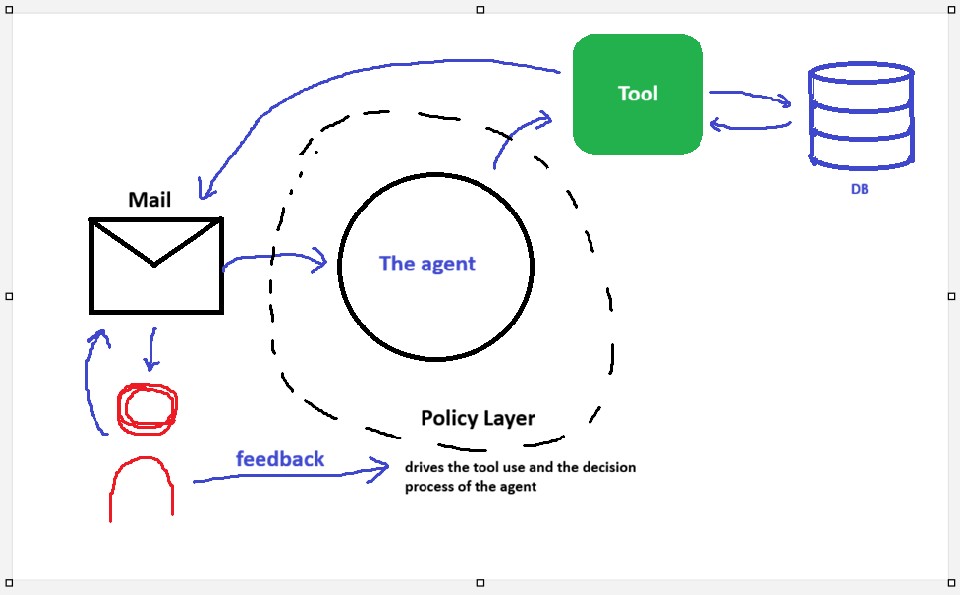
The mail-agent loop: an inbound email triggers a RAG search, the agent drafts a reply, and feedback on the reply feeds back into the loop — the mail-agent loop — an inbound email triggers the search, the agent writes a reply, and feedback on it closes the loop

So the question we kept coming back to: what does the policy layer look like?

Other policy layers

`CLAUDE.md`

The classic policy system is a CLAUDE.md file rewritten by the learning-mechanism layer. Each session, the agent reads CLAUDE.md and learns from past context. It is simple, but it has drawbacks. It is non-deterministic and non-explicable. If something failed, you cannot point to which part failed, why, and what to change next time. Even when the delta between two runs is positive, convergence can be slow and the limit sub-optimal.

GraphRAG approach

I played Outer Wilds (my favourite game, go play it, and do not get spoiled). In the game, a graph log system helps you remember information across sessions. Inspired by it, we built a graphRAG brain so the agent remembers what you did across sessions.

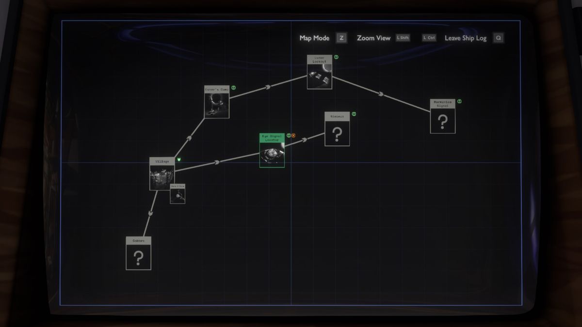
The Outer Wilds ship log, a graph of clues linked across sessions — the Outer Wilds ship log — clues stored as nodes and linked as you explore

In short, it is a graph-RAG CLAUDE.md. Nodes hold pieces of context that load only in certain situations. That way you can steer the agent toward certain actions in certain contexts.

the math of graph RAG, for the curious (optional)

Plain RAG embeds every chunk of context as a vector v ∈ ℝ^d, and for a query q it retrieves the k chunks whose embedding sits closest, usually by cosine similarity:

retrieve(q) = top-k_c [ (v_q · v_c) / (‖v_q‖ ‖v_c‖) ]

That treats context as a flat bag of chunks: no chunk knows about any other. Graph RAG adds the edges. The context is a graph G = (V, E), where nodes V are context pieces (entities, facts, a brain node) and edges E are the relations between them. Retrieval stops being a single similarity lookup and becomes a walk: seed on the query, then expand along edges to pull in the neighbourhood.

N_r(seed) = { v ∈ V : dist_G(seed, v) ≤ r }

The Microsoft GraphRAG paper adds one more step on top: run community detection (the Leiden algorithm) to partition V into clusters C₁, …, C_m of densely linked nodes, and pre-summarise each cluster. A global query is then answered from the community summaries rather than from raw chunks, which is why it beats flat RAG on questions that span the whole corpus. Leiden picks the partition that maximises modularity Q, the fraction of edges falling inside clusters minus what you would expect at random:

Q = (1 / 2m) · Σ_ij [ A_ij − (k_i k_j / 2m) ] · δ(c_i, c_j)

Here A_ij is the edge weight between nodes i and j, k_i the degree of node i, m the total edge weight, and δ(c_i, c_j) is 1 when the two nodes share a cluster and 0 otherwise. This is exactly what our brain does when it refactors semantically-close nodes together, and it is the reason a graph beats a flat file: retrieval follows the links instead of guessing from one similarity score.

Reference: Edge et al., From Local to Global: A Graph RAG Approach to Query-Focused Summarization (Microsoft Research, 2024).

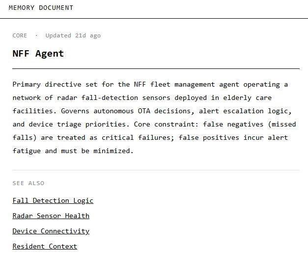
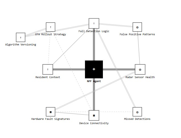
A single brain node holding a piece of markdown context — a single brain node — context loaded only in the situation it applies to

The graphRAG brain feature — the brain — nodes of context linked by the actions the agent takes

Why is this good? You use far less of the context window than a flat CLAUDE.md, and you get links between the actions the agent takes. First flaw: adding nodes. I set the brain to add a node whenever a conversation ends. Used a lot, here is what happens:

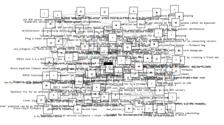
The brain feature crowded with too many nodes — that is a lot of nodes, and graphRAG gets lost

The fix: refactor nodes that are close semantically, and place them visually closer when they are close in meaning. This was inspired by graphify (graphify.net).

The problem remains: this is still hard to explain. The agent gets better context, but if an action or a chain of actions fails to reach its objective, you still do not know which part failed, so you do not know what to improve. And that assumes the agent knows its goal at all times. So we changed approach, moving closer to reinforcement learning.

The state-action graph for agents

This is where we arrived at the Agent driven Markov decision process (AD-MDP) method. If you want the correct math shenanigans that explain the theory behind this method, unfold the box below.

the math, for the curious (optional)

Formally, this is a partially observable Markov decision process (POMDP), a 7-tuple (S, A, T, R, Ω, O, γ). The states S are the graph nodes, the actions A the edges. The agent never sees the true fleet state s directly, only observations o ∈ Ω (a crash frame, a heap read, a missed heartbeat), so it is partially observable.

Taking action a in state s moves the system to s' with probability given by the transition function, and yields a cost (token burn, wall-clock, retries) via the reward function:

T(s' | s, a) = Pr(s_t+1 = s' | s_t = s, a_t = a)

R(s, a) = expected cost of running a in s

Because it cannot see s, the agent tracks a belief b, a probability distribution over states. A context tool (reading a device's heap) returns an observation o, and the belief is updated by Bayes' rule, the η normalising so it sums to one:

b'(s') = η · O(o | s', a) · Σ_s T(s' | s, a) · b(s)

The value of a belief is the best achievable discounted sum of future rewards, the Bellman equation over belief space, with discount γ ∈ [0, 1) weighting how much the far future counts:

V(b) = max_a [ Σ_s b(s) R(s, a) + γ Σ_o Pr(o | b, a) V(b') ]

Two things make our version tractable. We do not assume T, we estimate it online: run action a from state s many times, count how often it lands in s', and the empirical frequency converges to T(s' | s, a) (that is model-based RL). And the graph is sparse, each node wires to a handful of real actions, not the full |S| × |A| product, so the sums above run over a short list, not the whole fleet. The quality-gate layer tunes γ and the exploration rate, choosing how boldly the agent tries unseen edges to complete the map.

Reference: Sutton & Barto, Reinforcement Learning: An Introduction (2nd ed.).

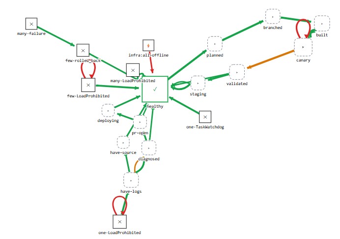
The state-action policy graph in the nff dashboard — the state-action policy graph in the dashboard — fleet states as nodes, agent actions as edges

In this weighted, directed graph, every state the agent can observe is a node. One node holds, for instance, the state multiple devices maintained, all online, all healthy, all tools healthy, ESP32 devices. Edges are the actions available in each state. An action can lead stochastically to another state. For example, upload a binary over the air to update firmware succeeds with probability P_ota, because the network can drop mid-upload and fail the flash.

To decide, the agent can call an action tool directly, or call a context tool (another MCP tool) that retrieves more context for a better decision, for instance, read a device's heap to confirm it crashed.

You start a nanoforgeflow session with a graph that works by default. It improves with use, absorbing your business logic to catch bugs that never trigger a concrete crash.

The goal of the graph is to self-improve. The agent improves two things: the decision-making, and the tools themselves.

Decision making

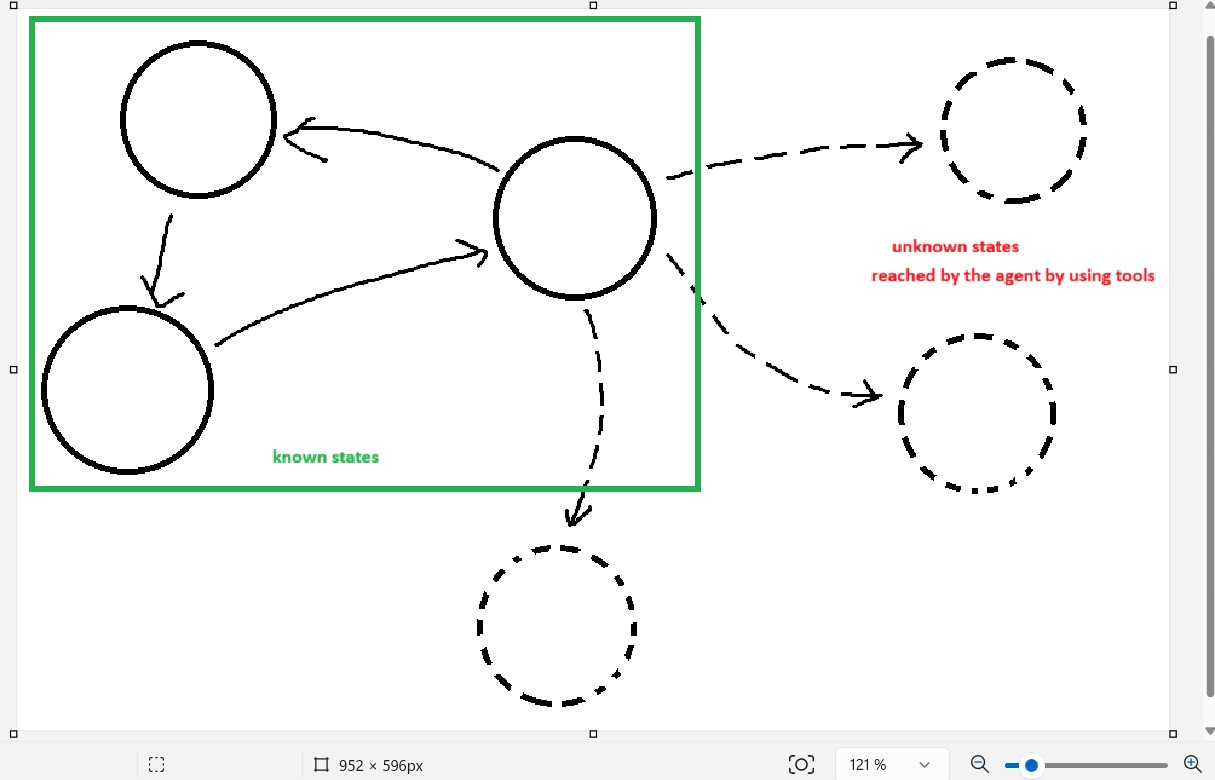
Clear decisions need a known environment. The agent can explore new actions in a state to see what they do to the system, learning them and completing the graph. With the whole map in front of it, it can apply classic exploitation algorithms from reinforcement learning: optimise the policy to maximise a value function, where the value function encodes the objectives x, y, z you want.

The agent exploring new actions to complete the state-action graph — exploration — the agent tries new actions in a state to learn their effects and complete the graph

What do the graph weights store as you run the agent through the policy graph? Three things. First, the probability of reaching state s' from state s by taking action a, measured by running action a many times and counting successes, which converges to the true probability. Second, the cost of the action: token burn, time, retry count. This lets you act differently when optimising for tokens, for time, or for agent calls. Third, the outcome: did this series of actions from this state succeed? This rewards taking action a or a' in a given state, and updates the policy downstream.

Tool-calling optimisation

Sometimes an action fails because the tool is called wrong, the right information is not passed. That is fixed by rewriting the function's description, or by correcting the tool itself.

Tool optimising

Google gave employees one day a week to build their own things. They came to the office, but could work on their own projects, that is how we got Google Suggest, the search autocomplete every browser uses today. Imagine the same for your agents. They can write new tools to shorten the path to reaching node x, y, z from another node, or, better, to explore more of their system, discovering things a human never imagined. Like a human, the quality-gate layer sees problems in the problem-solving flow, and can order a new function written to skip nodes and reach goals faster, or fix a function that failed on a bad call.

This is complementary to the brain context feature

You have to distinguish two things an agent does:

Actions that change the state of the system.
Actions that get the agent more context.

The policy graph handles the first, and keeps your system administered in a reliable, explicable way. The brain graph helps the agent decide. They are complementary. Remove the policy graph and decisions and tool calls become inexplicable. Remove the brain and you burn more tokens for lack of context, and you do not know where to get just the context you need.

About the quality-gate layer

All of this sets the framework for the agent to self-improve. The loop is not closed yet, that is the quality-gate layer, the feedback that improves the loop. Everything is tracked while an action runs: success rate, token burn, execution time, whether the action helped. The quality gate is an adversarial agent living one level above the nff worker agent. It looks at the worker's output and decides what to learn, what to enforce, and what to discard. Concretely, it changes the reward models and the exploration rate, which changes the agent's policy behaviour.

The user can queue tasks for the agent in a given order through an imperfect interface that exists today in the dashboard. A layer then translates user intent into graph-path requirements, which is really the value function.

Results

We ran the same batch of tasks under three policy layers, a flat CLAUDE.md, the brain feature, and POAD-MDP, with two agents driving: Claude and Codex. Two numbers matter: how many tasks land, and what they cost in tokens.

POAD-MDP clears the most tasks by a wide margin: 0.974 with Claude and 0.926 with Codex, up from 0.809 / 0.759 on the flat file, roughly +16 to +17 points. It is not the cheapest. The brain alone burns the fewest tokens but plateaus on the hard tasks. POAD-MDP spends more than the brain, yet still less than the flat file, while solving the tasks the other two leave on the table.

Claude Opus 4.8 Codex GPT-5.5

Task success rate

share of the batch solved. higher is better.
axis starts at 0.750.

0.750 0.875 1.000

0.809

0.759

0.835

0.819

0.974

0.926

Root md file Standalone Brain POAD-MDP

Token burn per batch

tokens spent on one whole batch of tasks. lower is better.
axis starts at 300k.

300k 450k 600k

545k

539k

325k

371k

421k

449k

Root md file Standalone Brain POAD-MDP

Metric	Agent	Root md file	Standalone Brain	POAD-MDP
Success rate	Claude Opus 4.8	0.809	0.835	0.974
Success rate	Codex GPT-5.5	0.759	0.819	0.926
Token burn / batch	Claude Opus 4.8	545k	325k	421k
Token burn / batch	Codex GPT-5.5	539k	371k	449k

One batch, two agents, identical task set. Success rate is the fraction of tasks solved; token burn is the total across the batch. Bold marks the best value on each row.

Limits of this approach, and what to improve

Decisions still rest on context, which is limited. Each tool consumes that context and drives the system into a new state. You cannot chain too many tools at once, but you can condense much of the prior history into a node and edge list.

This works well on the known graph we programmers laid down, because the tools were tailor-made for the cases shown here. The next step is obvious: make the state-action graph complete itself.

We will be releasing everything in open source in the coming days. If you want to get notified when we do, subscribe to the mailing list by signing in on nanoforgeflow.com/signup.

How we use this in nanoforgeflow

POAD-MDP operating a fleet in nanoforgeflow

This is not a thought experiment. It is how nff operates an ESP32-class fleet today. The three planes of the product map onto the graph.

Bench. A node is a board on the bench. Edges are compile, flash, and read serial. The agent loops those edges until the firmware works, learning which action clears which fault.
Ship. A git push is an edge that moves a device group from one firmware version to the next. The upload OTA edge carries the weight P_ota, so the agent stages the rollout instead of flashing the whole fleet at once.
Operate. A crash report is an observation that sharpens the belief over which fault a field device hit. The agent takes a context edge (resolve the backtrace, read the heap), then a state-changing edge (sign and push a fix), with dual-bank rollback as the recovery edge.

The weights are the fleet's own history: how often an OTA lands, what a retry costs in tokens and minutes, whether a given fix actually cleared the crash. The quality gate watches every OTA and tunes how boldly the agent explores an unproven edge on a device it cannot physically reach.

You start a session with a graph that already works for ESP32-class devices. It absorbs your business logic with use, catching the bugs that never throw a clean crash. That is the whole point: an operator that gets better at your fleet the longer it runs it.

Want to try it? nanoforgeflow.com — hardware, built instantly. no human in the loop.

← back